The arithmetic of chance

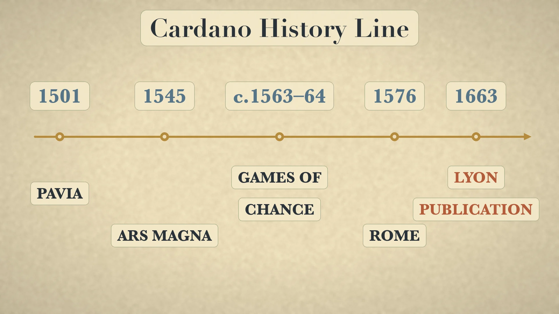
Gerolamo Cardano—also Girolamo Cardano, Latin Hieronymus Cardanus—was born in Pavia on 24 September 1501 and died in Rome on 21 September 1576. He was an Italian physician and mathematician whose life also involved gambling with cards, dice and chess. He worked and taught in Milan and Pavia, taught medicine at Pavia from 1543 to 1562, and transferred to a medical chair at Bologna in 1562. ^[1][2]

His Ars Magna appeared in 1545 and became important for its treatment of cubic and quartic equations. Liber de ludo aleae, the Book on Games of Chance, was probably completed by 1563 or written and revised in 1564; the date is reconstructed from an internal remark, so c.1563–1564 is more honest than a precise day. The work appeared posthumously in Lyon in the 1663 Opera Omnia. ^[3][5]

Historians commonly call the work the first systematic mathematical treatment, or first substantial study, of probability in games of chance. That is a retrospective description. Cardano did not have modern probability notation, and the manuscript contains correct and incorrect attempts. Its importance lies in counting outcomes and asking when a game is fair, not in making its author infallible. ^[3][4]

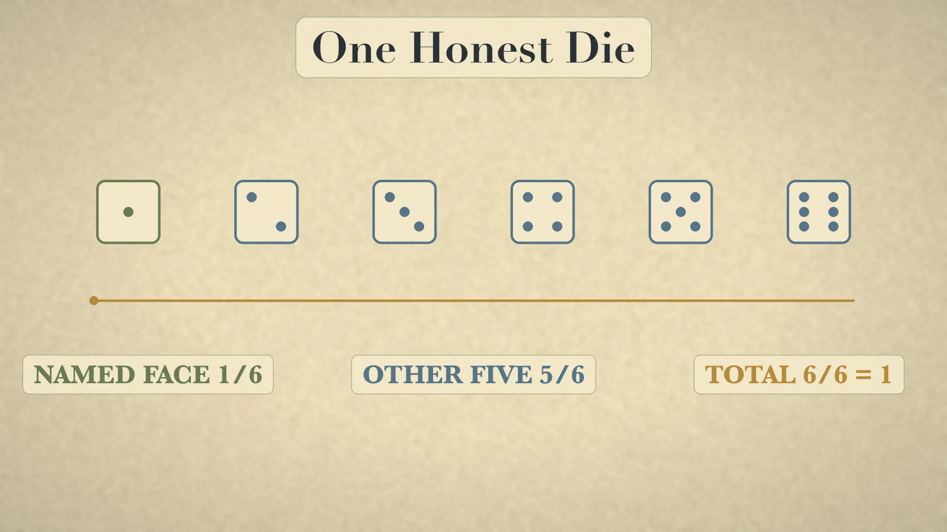
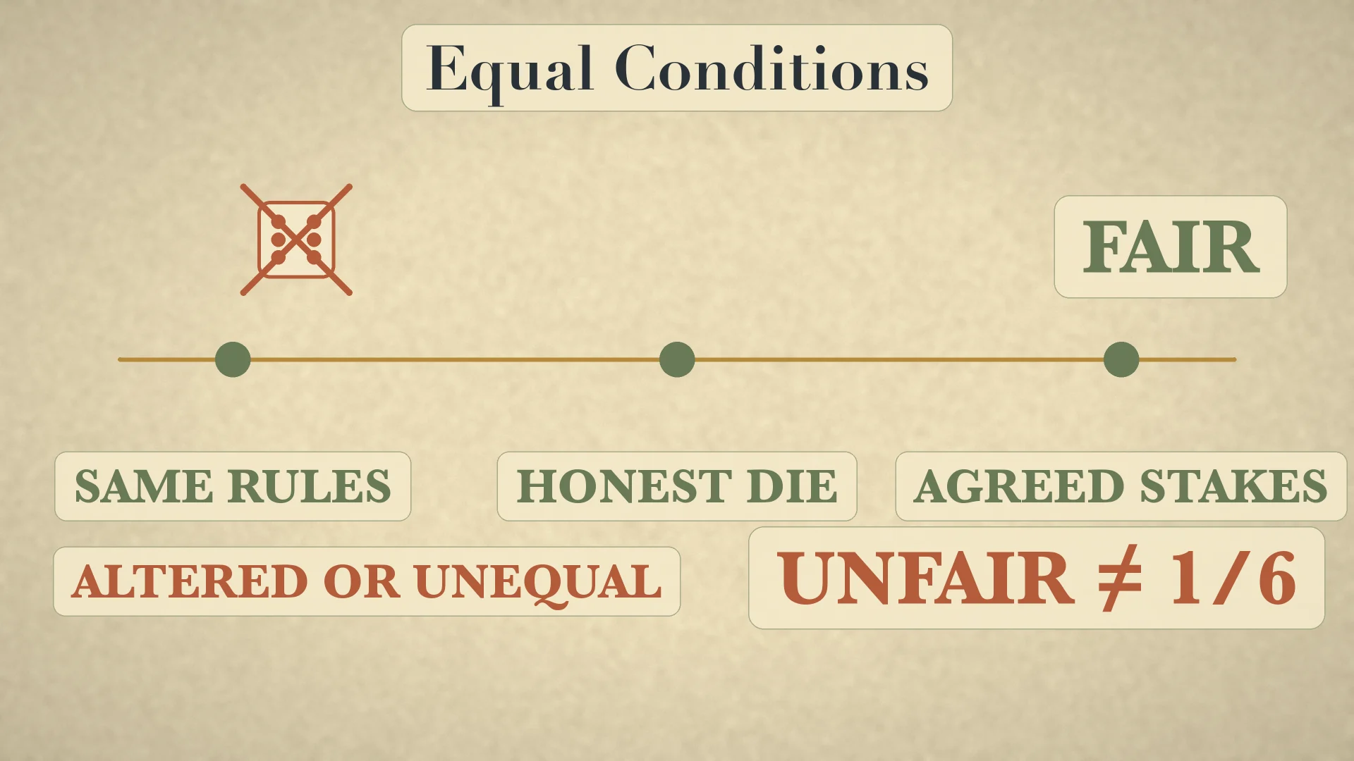
For one honest six-faced die, six faces are treated as equally possible. One named face has probability 1/6; the other five together have 5/6; all possibilities total 6/6=1. The calculation works because the outcome set and equal-likelihood assumption have been stated. If a die is altered, or a rule makes outcomes unequal, simply writing 1/6 is not justified.

Worked die example

1. Define the experiment: one roll of one honest six-faced die.
2. List the six outcomes: {1,2,3,4,5,6}.
3. Define success as rolling a 4; favourable cases = 1.
4. All equally possible cases = 6.
5. Probability is 1/6≈16.67%; probability of not rolling 4 is 5/6≈83.33%.
6. Check completeness: 1/6+5/6=6/6=1.

Cardano's equal-conditions principle belonged to games: comparable players, agreed rules and stakes, and honest equipment. The modern trading translation is procedural, not historical quotation: define outcomes consistently and do not assume trades are identically distributed when market process, costs or rules differ. Modern expectancy and percentage-risk rules must not be put into Cardano's mouth.

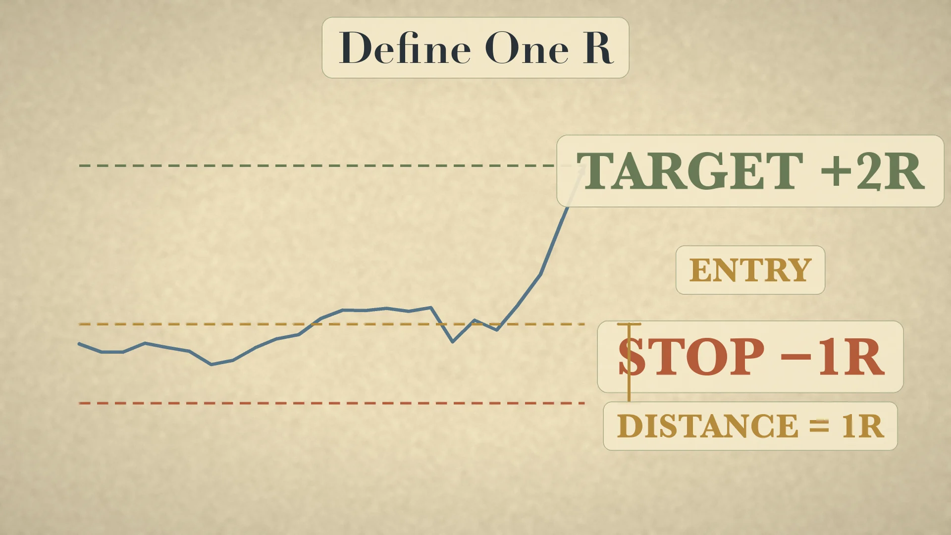
In the modern examples, R is the amount initially risked from entry to the stop. If entry is $50 and the predefined stop is $48, the price distance is $2. With 100 shares, 1R=$200 before costs. A stopped trade is −1R; a target twice the distance away at $54 is +2R. Expressing outcomes in R separates strategy arithmetic from account currency.

The definition must be fixed before the outcome. If the stop is moved from $48 to $46 after entry, the original $200 R no longer describes the realized exposure. If a gap exits at $47, the loss is −1.5R, not −1R. R is a bookkeeping unit, not a force that caps execution.

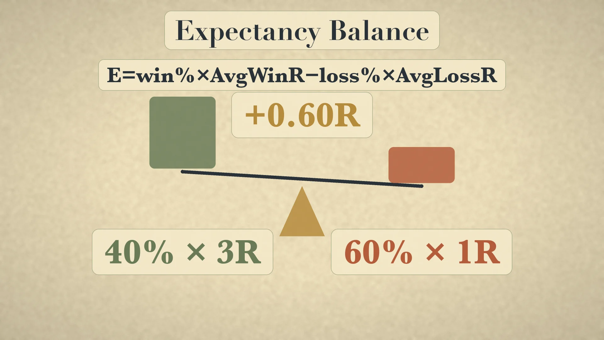
For a two-outcome model with no breakevens, E=P(win)×AvgWinR−P(loss)×AvgLossR and P(loss)=1−P(win). CME's worked values are 0.40×3R−0.60×1R=1.20R−0.60R=+0.60R per trade before commissions and slippage. This is a modelled average across repeated trades, not the result promised for the next one. ^[6]

Two strategies that expose the win-rate trap

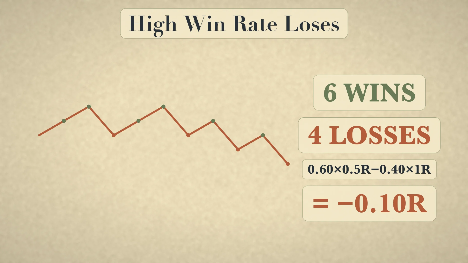
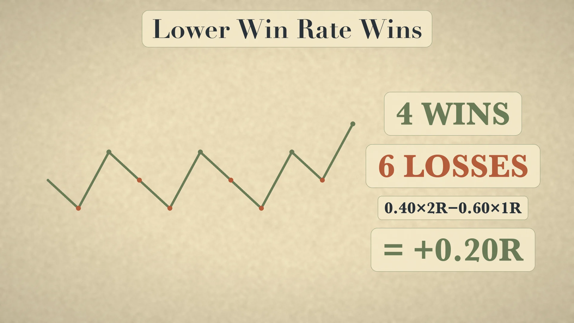
1. High-win example: P(win)=0.60, AvgWin=0.5R, P(loss)=0.40, AvgLoss=1R.
2. Calculate 0.60×0.5−0.40×1=0.30−0.40=−0.10R.
3. Lower-win example: P(win)=0.40, AvgWin=2R, P(loss)=0.60, AvgLoss=1R.
4. Calculate 0.40×2−0.60×1=0.80−0.60=+0.20R.
5. Conclusion: 60% wins can lose on average, while 40% wins can be positive before costs.

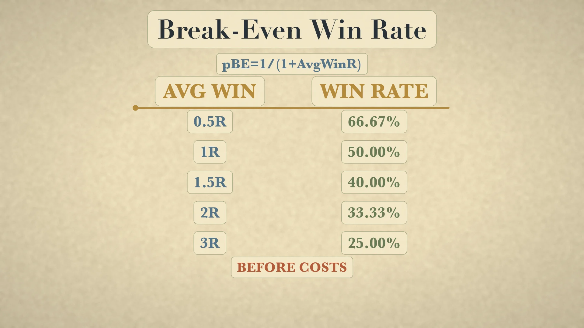
The break-even win rate follows by setting expectancy to zero with average loss fixed at 1R: pBE=1/(1+AvgWinR). For average wins of 0.5R, 1R, 1.5R, 2R and 3R, break-even rates are 66.67%, 50.00%, 40.00%, 33.33% and 25.00%. Costs raise every threshold because they reduce wins, enlarge losses, or both.

Worked break-even derivation

1. Set 0=p×W−(1−p)×1, where W is average win in R.
2. Expand: 0=pW−1+p.
3. Collect p: 1=p(W+1).
4. Solve: p=1/(W+1).
5. For W=2, p=1/3=33.33% before costs.

Under a stable process with independent or suitably well-behaved trials and finite expectation, the sample average tends toward the expected value as trial count grows. It does not say that a short run must resemble the average or that changing markets preserve an old edge. ^[7]

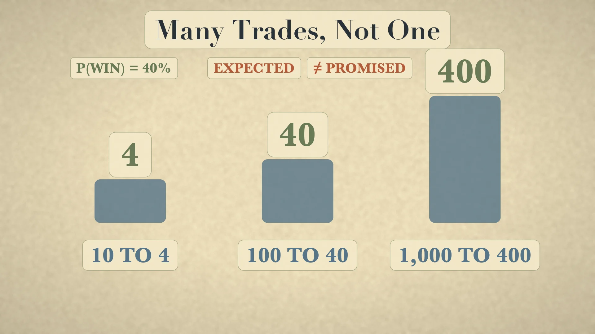
If P(win)=40%, expected wins are 10×0.40=4, 100×0.40=40, and 1,000×0.40=400. These are expected counts, not guarantees. A sequence of ten trades can contain two wins, seven wins or a long losing streak without changing the arithmetic of the assumed model. The crucial question is whether the assumed 40% remains stable enough to be useful.

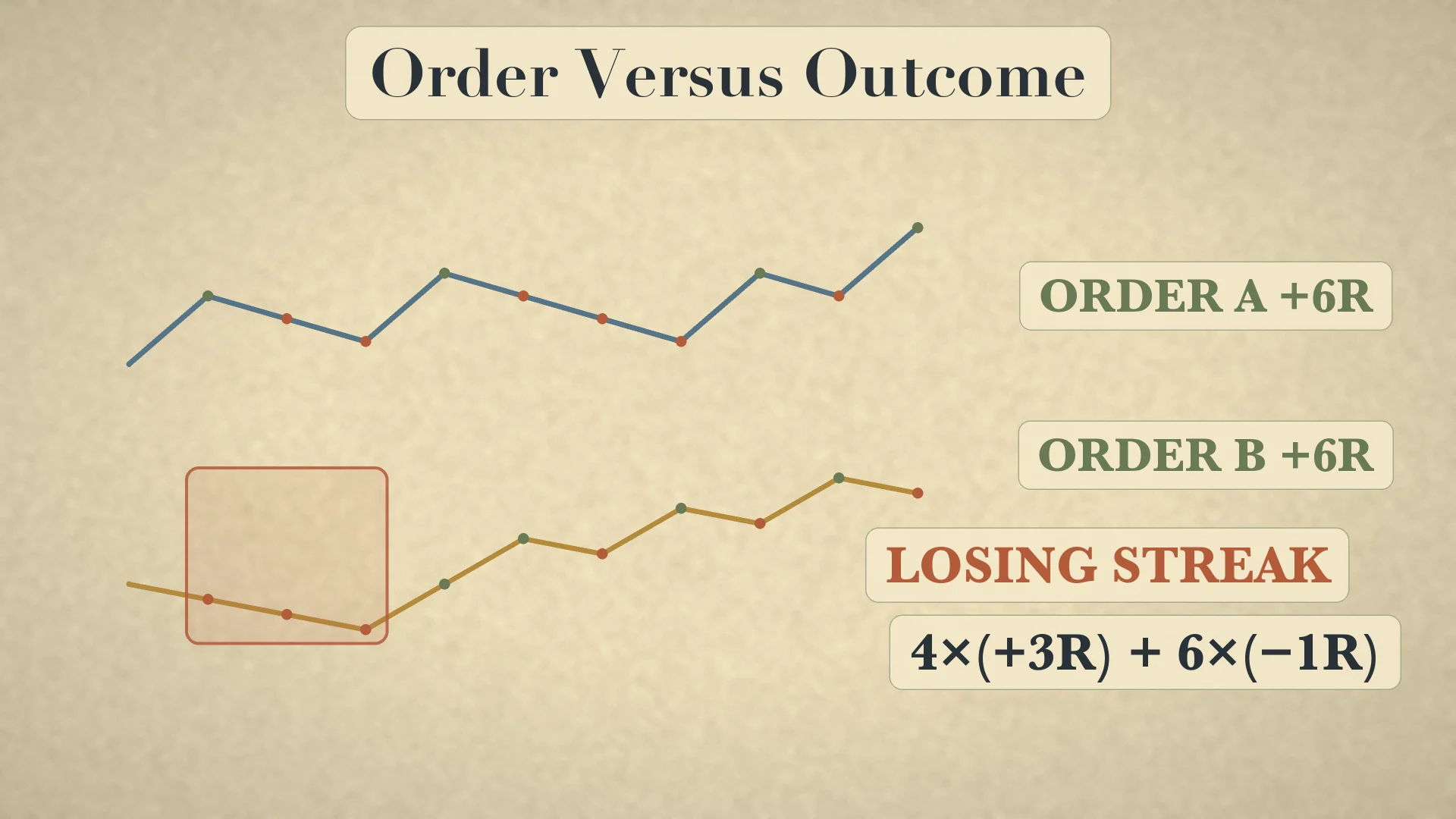
Order affects the path even when it does not affect the total. Ten trades containing exactly four +3R wins and six −1R losses total 12R−6R=+6R, whatever their order. But six losses first creates a −6R drawdown before the wins arrive. This is why expectancy, drawdown and sizing must be studied together.

Check expectancy against the sample total

1. The ten-trade sample has four wins and six losses, so observed win frequency is 40%.
2. Average win is 3R and average loss is 1R.
3. Formula expectancy is 0.40×3−0.60×1=+0.60R per trade.
4. Across ten trades, expected total at those exact sample frequencies is 10×0.60R=+6R.
5. Direct summation gives 4×3R−6×1R=+6R, so the two calculations reconcile.

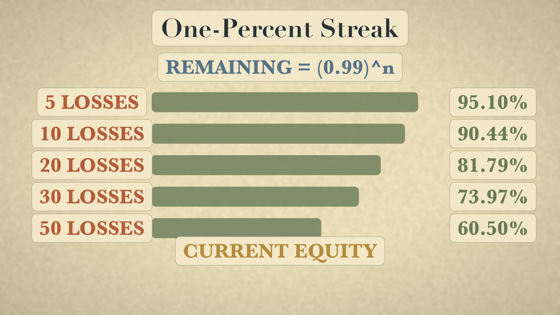
If every stopped trade loses fraction f of current equity, the remaining fraction after n consecutive losses is (1−f)^n. The multiplication uses current equity each time, not the original balance. With f=1%, five losses leave 0.99^5=95.10%; ten leave 90.44%; twenty 81.79%; thirty 73.97%; fifty 60.50%.

Worked 1% sequence

1. Start with $100,000.
2. After loss 1, equity is 100,000×0.99=$99,000.
3. After loss 2, equity is 99,000×0.99=$98,010.
4. After loss 5, equity is 100,000×0.99^5≈$95,099.
5. After loss 20, equity is 100,000×0.99^20≈$81,791.
6. The dollar loss shrinks with equity, but the account is still down about 18.21%.

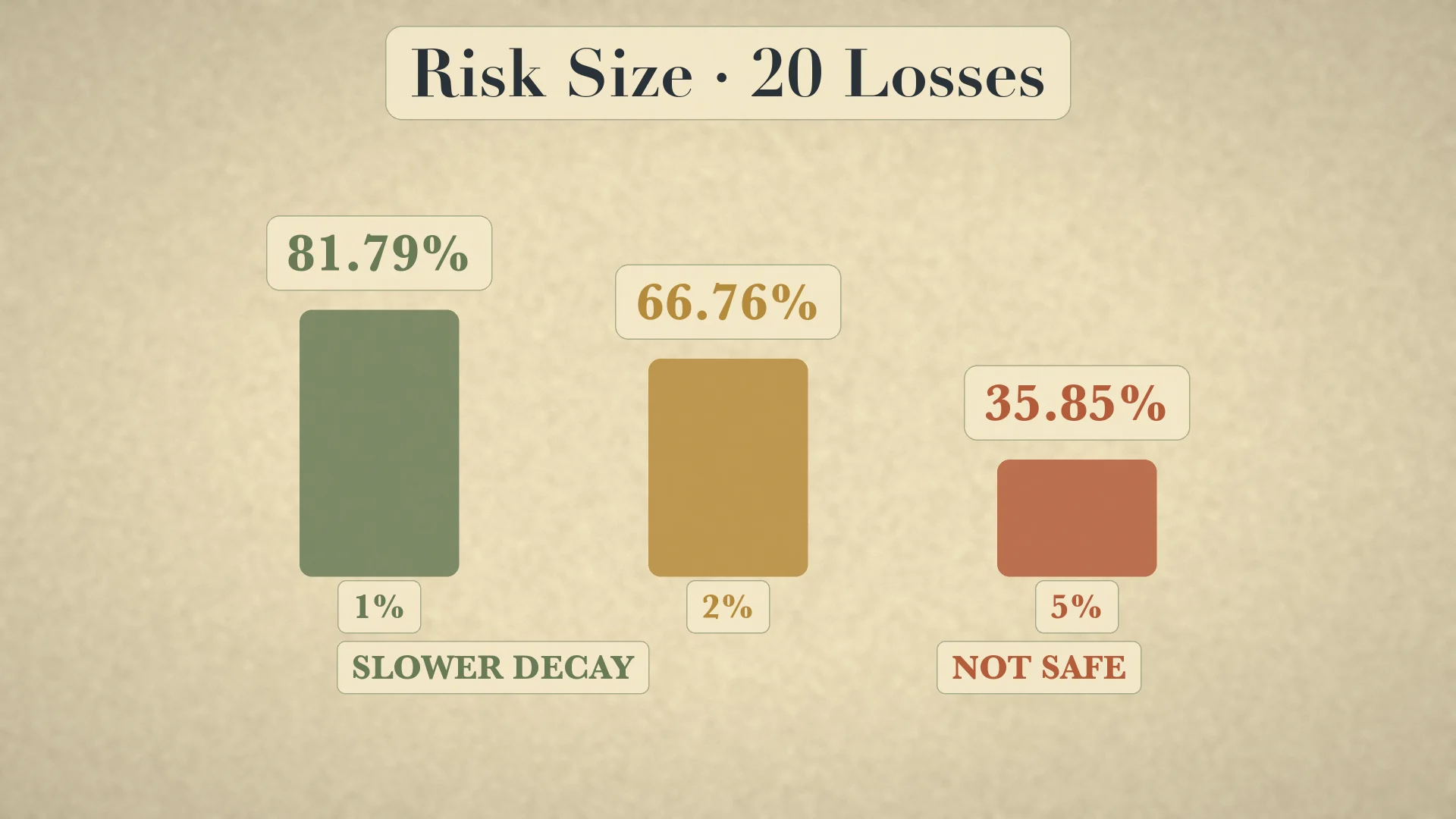
Risk fraction changes the decay dramatically. After 20 full-stop losses, 1% leaves 81.79%, 2% leaves 0.98^20=66.76%, and 5% leaves 0.95^20=35.85%. The correct label is slower decay, not safe. A gap, fee, leverage constraint or minimum contract size can produce a loss larger than f.

“Risk of ruin” is incomplete until ruin is defined and a model is stated. Possible thresholds include zero, a margin call, inability to trade the minimum size, or a maximum tolerable drawdown. The calculation also needs win probability, payoff distribution, dependence between trades, costs, leverage and position sizing. Change those assumptions and the result changes.

With pure percentage-of-current-equity sizing, no fees and no minimum size, repeated fixed-fraction losses approach zero mathematically without reaching it. A real account can still suffer practical ruin: margin rules can force liquidation, gaps can exceed the planned fraction, fees can dominate a small balance, and the estimated edge can disappear. The formula (1−f)^n therefore illustrates compounding; it is not a survival guarantee.

Define practical ruin before calculating it

1. Choose a threshold, such as a 30% maximum drawdown, a margin requirement, or the balance below which the minimum position cannot be traded.
2. State the position-sizing rule and whether risk is based on current or starting equity.
3. State the full payoff distribution, not only average win and loss.
4. Include commissions, slippage, gaps and leverage constraints.
5. Decide whether trials can be treated as independent and whether the estimated probabilities are stable.
6. Only then select an appropriate ruin model; no single percentage is valid without those inputs.

For example, an account may define practical ruin as falling below $7,500 because the minimum contract plus margin can no longer be supported. That threshold is reached long before mathematical zero. A second account trading divisible units without margin may have a different threshold. The phrase “risk of ruin” therefore names a modelling question, not a universal calculator button.

1. Define entry, stop and one R before the trade; do not rewrite them after seeing the outcome.
2. Record realized outcome in R, including slippage and fees.
3. From a sufficiently defined sample, calculate win frequency, average win R and average loss R.
4. Compute expectancy and a break-even rate; do not report win rate alone.
5. Inspect outcome order and losing streaks, not only the final sum.
6. Recalculate fixed-fraction drawdowns for several f values and define practical ruin.
7. Separate in-sample estimates from out-of-sample evidence and check whether process or costs changed.

Example: a chart setup has entry 50, stop 48 and educational target 54. One R is $2 per share; target is +2R. The setup is not attractive merely because the target is twice the stop. It still needs an independently estimated win frequency and actual average outcomes. If the observed win rate is 40% and average win really is 2R with average loss 1R, modelled expectancy is +0.20R before costs. If costs average 0.10R per trade, the remaining modelled edge is only +0.10R.

Costs can also move the break-even rate. If a nominal 2R winner nets only 1.9R after average costs while a nominal 1R loss becomes 1.1R, then at a 40% win rate expectancy is 0.40×1.9−0.60×1.1=0.76−0.66=+0.10R. A further 0.10R deterioration removes the modelled edge. Small assumptions matter when expectancy is small.

Common mistakes are assuming all market outcomes are equally likely, changing R after the fact, using target size instead of realized average win, confusing positive expectancy with a next-trade forecast, treating expected counts as promised counts, and calling 1% sizing ruin-proof. This article can verify arithmetic only. It cannot prove a live edge, predict sequence, model a broker's exact gaps or guarantee survival; those require trade-level data, explicit costs and out-of-sample testing.